Table of Contents

1. Problem Statement
2. Model
3. Dataset
4. Model Development
5. Set up Model Training
6. Training
7. Detection
8. Future Scope
9. Leaving Note
10. Contact

Problem Statement

The assignment is to create a network that can perform 3 tasks simultaneously:

1. Predict the boots, PPE, hardhat, and mask if any present in the image
2. Predict the depth map of the image
3. Predict the Planar Surfaces in the region

The strategy is to use pre-trained networks and use their outputs as the ground truth data:

• Midas Depth model for generating depth map
• Planercnn network for identifying Plane surface
• Yolov3 network for object detection

Model

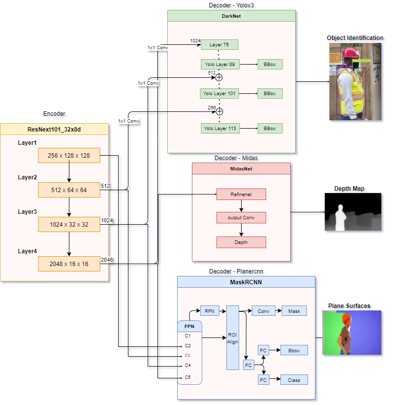
The Network is of Encoder-Decoder Architecture

• Layers: 1056
• Parameters: 23.7m
• Min loss: 7
• Trained Model weight - Download

Dataset

The data used for the training of the model is as below.

Download Data

The high level steps taken to create the dataset is as below:

1. Collect images from different website of people wearing hardhat, masks, PPE and boots.
2. For object detection, use YoloV3 annotation tool to draw bounding box for the labels.
3. Use MidasNet by Intel to generate the depth for the images
4. Use Planercnn to generate plane segmentations of the images

A detailed explanation and code can be found in this Repo

Issues faced

• By default Planercnn gives the following outputs for each input image
  • Image.png
  • Plane_parameters.npy
  • Plane_masks.npy
  • Depth_ori.png
  • Depth_np.png
  • Segmentation.png
  • Segmentation_final.png
• For our purpose we do not need the depth prediction of the Planercnn, therefore we can omit depth*.png,image.png is same the input image hence we can omit that also.so for our use case, plane_parameters.npy, plane_masks.npy and segmentation_final.png is only required
• We frequently run outo Disk space as *.npy files are heavy, so to handle it i replace both the np.save() of the .npy files with a single np.savez_compressed() line, This helps to save disk space as well as store numpy files
• The output files are saved with index number rather than their actual names, this can be handled by replacing the visualizebatchPair() parameter from the index number to the image filename in Visualise_utils.py

Additional Data

Download link

• Additional data for the training of Planercnn has been created
• A Youtube Video of indoor surfaces is used to create images by generating frame every 0.5 second,the frames are then used to generate the Planercnn output.

Model Development

In this section I will explain the steps taken to reach the final trainable model. Significant amount of time was invested in the initial to read all the research papers of each model and get a understanding of their architecture, this would enable us to split their encoder from their decoder.

1. Step 1: To define the high outline of the final model and then start to give definition for each of its components

• The structure of the model defined is as below

  
      class VisionNet(nn.Module):
  
        '''
          Network for detecting objects, generate depth map and identify plane surfaces
        '''
  
        def __init__(self,yolo_input,midas_input,planercnn_input):
          super(VisionNet, self).__init__()
          """
            Get required configuration for all the 3 models
              
          """
          self.yolo_params = yolo_input
          self.midas_params = midas_input
          self.planercnn_params = planercnn_input
              
          self.encoder = Define Encoder()
  
          self.plane_decoder = Define Plane decoder(self.planercnn_params)
  
          self.depth_decoder = Define Depth decoder(self.midas_params)
              
          self.bbox_decoder =  Define Yolo decoder(self.yolo_params)
              
  
        def forward(self,x):
  
          x = self.encoder(x)
  
          plane_out = self.plane_decoder(x)
  
          depth_out = self.depth_decoder(x)
              
          bbox_out = self.bbox_decoder(x)
  
          return  plane_out, bbox_out, depth_out
  
  

1. Step 2: Define Encoder Block
   • The 3 different encoder block in each of the networks:
     • MidasNet - ResNext101_32x8d_wsl
     • Planercnn - ResNet101
     • Yolov3 - Darknet-53
   • My initial thoughts was to use Darknet as the base encoder, as the similar accuracy as ResNet and it is almost 2x faster based on performance on ImageNet dataset, but the downside of it is compartively complex to separate only the config of Darknet from Yolov3 config and then run the same code blocks from Yolov3 from model definition and forward method, This could mean i have to recreate those code blocks with changes so that only Darknet encoder is proccesed. Hence, as the enocder-decoder of Yolov3 is tighly coupled in code i decided against using it.
   • On other two options, I had tried both of them separately as the encoder blocks, based on the benchmarks ResNext-101 has perfomed better than Resnet-101 and ResNext WSL is maintained by facebook and are pre-trained in weakly-supervised fashion on 940 million public images with 1.5K hashtags matching with 1000 ImageNet1K synsets, followed by fine-tuning on ImageNet1K dataset, So the below ResNext block is used as enoder with the pretrained weights

         resnet = torch.hub.load("facebookresearch/WSL-Images", "resnext101_32x8d_wsl")
   

• The encoder is defined with 4 pretrained layers

    def _make_resnet_backbone(resnet):
        pretrained = nn.Module()
        pretrained.layer1 = nn.Sequential(
            resnet.conv1, resnet.bn1, resnet.relu, resnet.maxpool, resnet.layer1
        )
        pretrained.layer2 = resnet.layer2
        pretrained.layer3 = resnet.layer3
        pretrained.layer4 = resnet.layer4
        return pretrained
  

1. Step 3: Define Depth decoder block

• This was pretty direct reference form the midasnet block excluding only the pretrained encoder

    class MidasNet_decoder(nn.Module):
    """Network for monocular depth estimation.
    """
  
    def __init__(self, path=None, features=256,non_negative=True):
        super(MidasNet_decoder, self).__init__()
        """Init.
  
        Args:
            path (str, optional): Path to saved model. Defaults to None.
            features (int, optional): Number of features. Defaults to 256.
  
        """
        self.scratch = _make_encoder_scratch(features)
  
        self.scratch.refinenet4 = FeatureFusionBlock(features)
        self.scratch.refinenet3 = FeatureFusionBlock(features)
        self.scratch.refinenet2 = FeatureFusionBlock(features)
        self.scratch.refinenet1 = FeatureFusionBlock(features)
  
        self.scratch.output_conv = nn.Sequential(
            nn.Conv2d(features, 128, kernel_size=3, stride=1, padding=1),
            Interpolate(scale_factor=2, mode="bilinear"),
            nn.Conv2d(128, 32, kernel_size=3, stride=1, padding=1),
            nn.ReLU(True),
            nn.Conv2d(32, 1, kernel_size=1, stride=1, padding=0),
            nn.ReLU(True) if non_negative else nn.Identity(),
        )
  
  
    def forward(self, *xs):
        """Forward pass.
  
        Args:
            x (tensor): input data (image)
  
        Returns:
            tensor: depth
        """
  
        layer_1, layer_2, layer_3, layer_4 =  [xs[0][i] for i in range(4)]
  
  
        layer_1_rn = self.scratch.layer1_rn(layer_1)
        layer_2_rn = self.scratch.layer2_rn(layer_2)
        layer_3_rn = self.scratch.layer3_rn(layer_3)
        layer_4_rn = self.scratch.layer4_rn(layer_4)
        #print('layer_4_rn',layer_4_rn[0][0])
  
        path_4 = self.scratch.refinenet4(layer_4_rn)
        path_3 = self.scratch.refinenet3(path_4, layer_3_rn)
        path_2 = self.scratch.refinenet2(path_3, layer_2_rn)
        path_1 = self.scratch.refinenet1(path_2, layer_1_rn)
  
        out = self.scratch.output_conv(path_1)
        #print('out',out.size(),out)
        #print('out squeeze',torch.squeeze(out, dim=1).size(),torch.squeeze(out, dim=1))
  
        final_out = torch.squeeze(out, dim=1)
  
        return final_out
  

1. Step 4: Define Object detection decoder block

• yolov3 custom cfg file had to be changed to omit the encoder part of the network and retain only the decoder part
• Darknet-53 is feature extrator that extends upto the 75th layers in the yolo network, also a key point to note is there are 3 skip connection from the Darknet encoder to decoder for object detection
• A print of the layer name with the sizes give understanding of the each layer along with their output shape FILE
• To pass the output from the encoder layers to the corresponding layer in Yolo, a 1x1 convolution was used
  • Encoder layer 2 output –> Yolo 36th layer
  • Encoder layer 3 output –> Yolo 61st layer
  • Encoder layer 4 output –> Yolo 75th layer

      init:
      self.conv1 = nn.Conv2d(in_channels=2048, out_channels=1024, kernel_size=(1, 1), padding=0, bias=False)
      self.conv2 = nn.Conv2d(in_channels=1024, out_channels=512, kernel_size=(1, 1), padding=0, bias=False)
      self.conv3 = nn.Conv2d(in_channels=512, out_channels=256, kernel_size=(1, 1), padding=0, bias=False)
    
      forward:
      Yolo_75 = self.conv1(layer_4)
      Yolo_61 = self.conv2(layer_3)
      Yolo_36 = self.conv3(layer_2)
    
    

• The Darknet layer configuration post the custom changes can ve viewed from this CUSTOM FILE

1. Step 5: Define Plane segmentation decoder block
   • Planercnn is built of MaskRcnn network which consists of resnet101 as the backbone for feature extractor and then it is followed by FPN,RPN and rest of the layers for detections
   • The first 5 layers(C1 - C5) of FPN are directly from the resnet101 block, which i changed to connect to our layers from the custom encoder block (note: C1 & C2 together form the layer 1 of our ResNext101 Encoder)
     • Encoder layer 1 output –> FPN C1 layer
     • Encoder layer 2 output –> FPN C2 layer
     • Encoder layer 3 output –> FPN C3 layer
     • Encoder layer 4 output –> FPN C4 layer
   • Key concept in Planercnn integration is that the default nms and ROI is coplied on the torch verions 0.4, which is incompatible with other decoder modules which use latest torch version, to handle this the default nms was replaced with the nms from torchvision and the ROI Align buit on pytorch(link) was used
   • One key issue faced during training is of gradient explosion after one iteration of the model train, post significant time debugging the reason in due to the replacement of the resnet101 directly with the custom encoder blocks, the solution for the issue was to retain the resnet101 structure but to replace the value of tht corresponding layers in FPN with enocder layers in the forward method
2. Step 6: The Trainable model

• The Final trainable version of the model is as below

    class VisionNet(nn.Module):
  
      '''
        Network for detecting objects, generate depth map and identify plane surfaces
      '''
  
      def __init__(self,yolo_cfg,midas_cfg,planercnn_cfg,path=None):
        super(VisionNet, self).__init__()
        """
          Get required configuration for all the 3 models
            
        """
        self.yolo_params = yolo_cfg
        self.midas_params = midas_cfg
        self.planercnn_params = planercnn_cfg
        self.path = path
  
        use_pretrained = False if path is None else True
  
        print('use_pretrained',use_pretrained)
        print('path',path)
            
        self.encoder = _make_resnet_encoder(use_pretrained)
  
        self.plane_decoder = MaskRCNN(self.planercnn_params,self.encoder)
  
        self.depth_decoder = MidasNet_decoder(path)
  
        self.bbox_decoder =  Darknet(self.yolo_params)
  
        self.conv1 = nn.Conv2d(in_channels=2048, out_channels=1024, kernel_size=(1, 1), padding=0, bias=False)
        self.conv2 = nn.Conv2d(in_channels=1024, out_channels=512, kernel_size=(1, 1), padding=0, bias=False)
        self.conv3 = nn.Conv2d(in_channels=512, out_channels=256, kernel_size=(1, 1), padding=0, bias=False)
            
        self.info(False)
  
      def forward(self,yolo_ip,midas_ip,plane_ip):
  
        x = yolo_ip
        #x = midas_ip
  
        # Encoder blocks
        layer_1 = self.encoder.layer1(x)
        layer_2 = self.encoder.layer2(layer_1)
        layer_3 = self.encoder.layer3(layer_2)
        layer_4 = self.encoder.layer4(layer_3)
  
        Yolo_75 = self.conv1(layer_4)
        Yolo_61 = self.conv2(layer_3)
        Yolo_36 = self.conv3(layer_2)
  
        if plane_ip is not None:
          plane_ip['input'][0] = yolo_ip
          # PlaneRCNN decoder
          plane_out = self.plane_decoder.forward(plane_ip,[layer_1, layer_2, layer_3, layer_4])
        else:
          plane_out = None
  
        if midas_ip is not None:
          # MiDaS depth decoder
          depth_out = self.depth_decoder([layer_1, layer_2, layer_3, layer_4])
        else:
          depth_out = None
  
        #YOLOv3 bbox decoder
        if not self.training:
          inf_out, train_out = self.bbox_decoder(Yolo_75,Yolo_61,Yolo_36)
          bbox_out=[inf_out, train_out]
        else:
          bbox_out = self.bbox_decoder(Yolo_75,Yolo_61,Yolo_36)
  
        return  plane_out, bbox_out, depth_out
  
      def info(self, verbose=False):
        torch_utils.model_info(self, verbose)
  
  

Set up Model Training

1. Step 1: Define input parameters for training
   • As each of the 3 network have their own multiple default parameters for decoder configurations and data preproccessing, I combined the Arg parser of all the 3 decoders into single file options.py
   • This ensures we able to pass the required input parameters including weights path for each of the decoders separately
2. Step 2: Define Skeleton
   • Midasnet repo is defined only for inference and train for custom data is not part of it
   • Planercnn repo is pretty huge and structure for train dataset and process for generating the dataset is complex and time taking
   • Yolov3 repo has defined the training process
   • hence used the Yolov3 training code as reference for the training the model
3. Step 3: Data loader
   • Defined different dataset for train and test from the split train.txt and test.txt file from the dataset
   • included the data tranformations from the 3 decoders
   • Additionaly for Planercnn training loaded the segmentation_final.png and plane_parameters.npy & plane_masks.npy files and similarly for depth training loaded the depth map images
   • Code blocks of Planercnn is defined only to work for batch size of 1, hence any other batch size > 1 will not work with the current code base
4. Step 4: Loss function
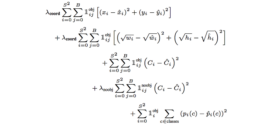
   • Object detection - the compute loss method of the yolov3 code base to calculate the loss for the object detection network, The complete loss equation as below

   

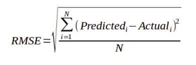
   • Depth Estimation - to compare the predicted depth map with that of the target image a combination of the below two loss is use
     • RMSE(Root Mean Square Error): RMSE helps to cut the large errors interms of difference in the intensity of the pixels of the image
     • SSIM(structural similarity index measure): SSIM helps to also measure the structural differences between the predicted and the acutal depths and also to punish noises in the prediction
     • Depth_loss = RMSE + SSIM
   • Plane Segmentation - to define loss for plane segmentation
     • The predefined loss function in planercnn uses cross_entropy loss to compare rpn_class and rpn_bbox
     • MSE(Mean Squared Error) is used to directly compare the plane_parameters.npy & Plane_masks.npy with the predicted np arrays, MSE performs better at pixel level comparison
     • SSIM is also used to compare the segmentation image predicted with target image
     • Plane_loss = computed_loss + MSE_Loss + SSIM
   • overall loss

   all_loss = (add_plane_loss * plane_loss) + (add_yolo_loss * yolo_loss) + (add_midas_loss * depth_loss)

5. Step 5: Optimizer
   • Stochastic Gradient Descent(SGD) is used as the default optimizer with the below params
     • start lr : 0.01
     • Final lr : 0.0005
     • momentum : 0.937
     • weight_decay : 0.000484
   • Scheduler : Lambda lr

Training

1. One key issue faced during the training for frequent running out of memory, below steps were used to handle the same - Clear torch cuda cache at the end of each epoch - use python grabage collector at the end of each training iteration to clear the space of variables that are no longer required
2. Trining on small resolution images - Initial few epochs was performed on 64x64 images but this could only be done for Object detection and depth map as planercnn accepts image only with minimum size of 256
3. Optimum resolution as which the entire model could train is 512 x 512, most of the epchs are run with this resolution
4. The additional data was used for training the planercnn mode separately

5. The time taken for each epoch initial was around 1.15 hours, this was reduced after standardising the image scales in all decoder to 512, (Planercnn had 480*640 and midas was working with 384*384). The time taken for each epoch right now is 40-50 min

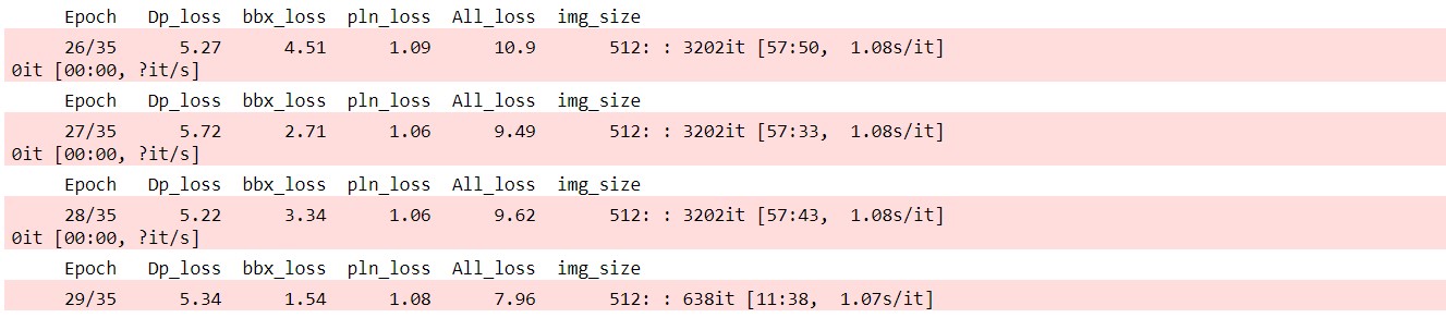
6. Part 1 training we could see the overall loss decreasing as the model is getting trained, The initial for epoch 0 was at 21. (notebook)

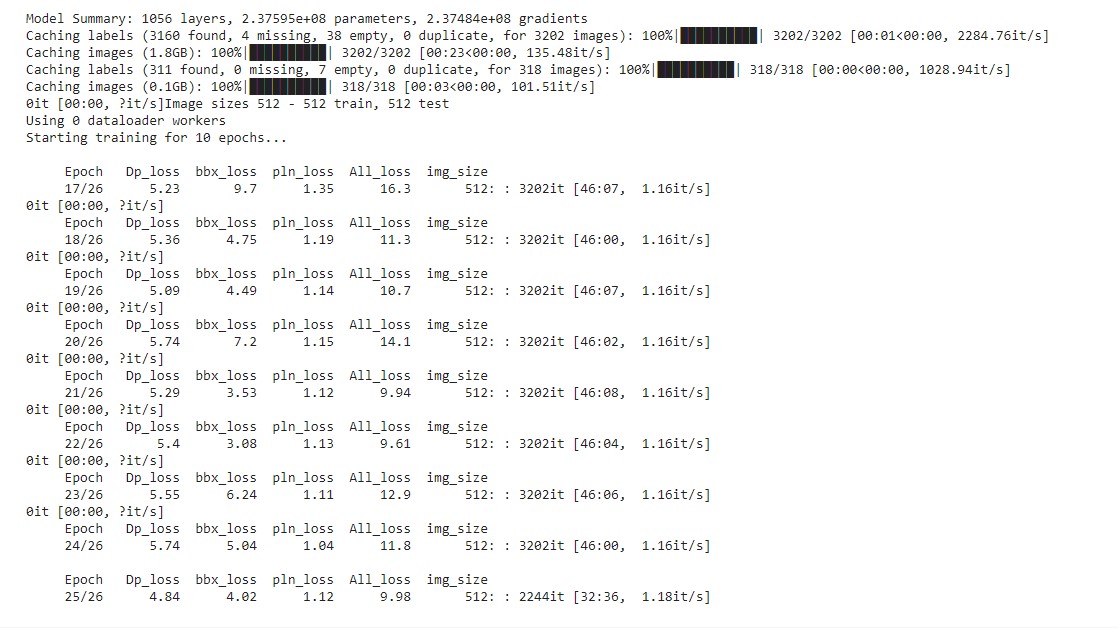
1. Part 2 training the overall loss further reduced in subsquent epochs to 7 (notebook)

Detection

• Detections can be performed using the detection.py with the below code notebook

python detection.py

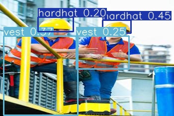
• Example:
  • Object Detection output:

  

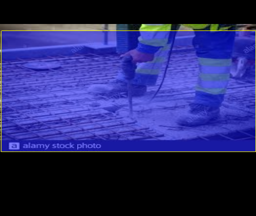
  • Midas detection

  

  • Plane segmentation (create test folder in project_vision folder to save plane images during training also)

  

Future Scope

• Definitely there huge scope for model improvement, its current performance is not upto the mark
• revist the image augmentation strategies to define something which suits for all 3 tasks
• Collect more data and train the model for more epochs
• Play around with loss function

Leaving Note

• My journey of the capstone project is best summarised with the image below
• There were many days were I thought I would never reach a trainable model but to progress till here i consider it a success, and I take immense confidence out from this project that now i would be able to deal with any difficult complex problem if I am persistant
• Thanks to Rohan Shravan for being the best mentor and Zoheb for all the immense learning in past 4 months
• Hope to See you in Phase 2 !!!

Contact

For any further clarification or support kindly check my github repo or contact